Tutorials

Quick-start

In this tutorial, we will demonstrate:

How to initialise the emulator
How to compute multipoles for the standard \(\Lambda\)CDM cosmology

Let’s begin by importing comet along with the necessary libraries:

from comet import comet
import numpy as np
import matplotlib.pyplot as plt

When initialising the emulator, we need to select a specific perturbative model. Currently, COMET supports three options:

Effective Field Theory of Large-Scale Structure: 'EFT'
Model with non-perturbative damping function: 'VDG_infty'
Real-space model: 'RS'

For a detailed overview of the available models, please check here. Each of these models comes with two separate emulators, based on whether the user wants to include the effect from massive neutrinos or not. These can be selected by using the model identifier specified above (e.g. EFT) or by further attaching the string _nonu (e.g. EFT_nonu). Additionally, we can configure COMET to use either:

\(\mathrm{Mpc}\) units (use_Mpc=True, default option)
\(h^{-1}\,\mathrm{Mpc}\) units (use_Mpc=False)

All non-dimensionless quantities will be assumed to be in the chosen unit system and returned accordingly.

Let’s now define an emulator object for the EFT model without massive neutrinos using \(h^{-1}\,\mathrm{Mpc}\) units:

EFT = comet(model='EFT_nonu', use_Mpc=False)

Before making predictions for a given cosmological model, we need to specify the fiducial background cosmology. This is essential for computing Alcock-Paczynski distortions. To set up the fiducial cosmology in COMET, we use the function define_fiducial_cosmology:

# This assumes by default a LCDM cosmology; for other
# options, see the in-depth examples below.
params_fid = {'h': 0.695, 'wc': 0.11544, 'wb': 0.0222191, 'z': 0.57}

EFT.define_fiducial_cosmology(params_fid=params_fid)

The function Pell, which returns the power spectrum multipoles, requires three main inputs:

k: the scales at which to compute the multipoles, given in the appropriate units
params: the input dictionary, including cosmological, bias, and RSD parameters
ell: the Legendre multipole order (can be either 0, 2, 4, or a list of values, e.g. [0, 2, 4])

The parameter dictionary must include all shape parameters, specifically:

Cold dark matter densities (wc)
Baryon density (wb)
Scalar spectral index (ns)

For a flat \(\Lambda\)CDM cosmology, we also have to specify the evolution parameters:

Dimensionless Hubble parameter (h)
Scalar spectral amplitude (As)
Redshift (z)

For alternative cosmologies and advanced configurations, refer to later sections of this tutorial.

# Let's create a parameter dictionary
params = {}

# We always need to specify the shape parameter values, e.g.
params['wc'] = 0.11544
params['wb'] = 0.0222191
params['ns'] = 0.9632

# For a LCDM cosmology, we also need:
params['h']  = 0.8
params['As'] = 2.3 # As is in units of 1e-9
params['z']  = 0.6

Finally, we define the values of the bias parameters. The complete list of parameters along with a brief explanation and their dictionary keywords can be found here. In the following we only specify values for the linear and quadratic bias (all other parameters are automatically set to zero):

params['b1'] = 2.0
params['b2'] = -0.5

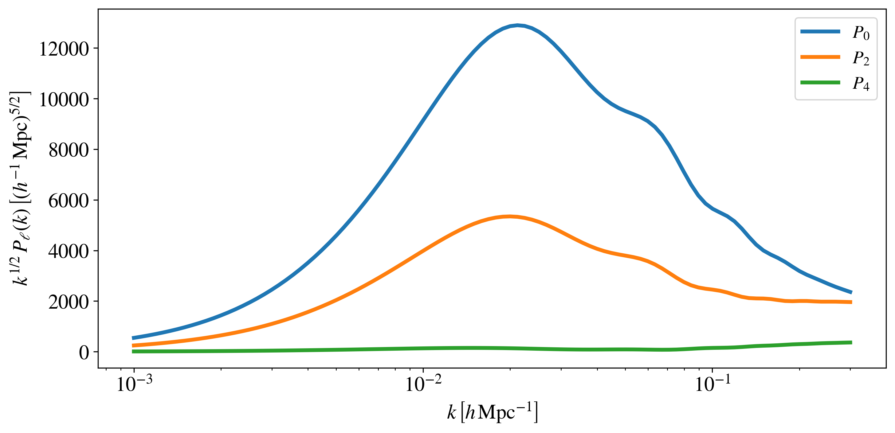
Now, let’s compute the monopole (ell=0), quadrupole (ell=2) and hexadecapole (ell=4) for a range of scales from \(0.001\,h\,\mathrm{Mpc}^{−1}\) to \(0.3\,h\,\mathrm{Mpc}^{−1}\,\):

k_hMpc = np.logspace(-3, np.log10(0.3), 100)

# The extra argument `de_model` is necessary to specify
# that we are working with a LCDM cosmology. In the next
# sections we will show how to work with other settings.
Pell_LCDM = EFT.Pell(k=k_hMpc, params=params, ell=[0,2,4], de_model='lambda')

The output of the Pell function is given as a dictionary:

print(Pell_LCDM.keys())
>> dict_keys(['ell0', 'ell2', 'ell4'])

Finally, we can access our results and plot them as follows:

fig = plt.figure(figsize=(10,5))
ax = fig.add_subplot(111)
ax.semilogx(k_hMpc, k_hMpc**0.5 * Pell_LCDM['ell0'], c='C0', ls='-', lw=3, label=r'$P_0$')
ax.semilogx(k_hMpc, k_hMpc**0.5 * Pell_LCDM['ell2'], c='C1', ls='-', lw=3, label=r'$P_2$')
ax.semilogx(k_hMpc, k_hMpc**0.5 * Pell_LCDM['ell4'], c='C2', ls='-', lw=3, label=r'$P_4$')
ax.set_xlabel(r'$k \, \left[h\,\mathrm{Mpc}^{-1}\right]$')
ax.set_ylabel(r'$k^{1/2} \, P_{\ell}(k) \, \left[(h^{-1}\,\mathrm{Mpc})^{5/2}\right]$')
ax.legend()
plt.tight_layout()
plt.show()

Massive neutrinos

To work with massive neutrinos, we need to use a different sets of emulators that have been trained also in terms of the total neutrino mass Mnu. In this case, simply specify the model name without the '_nonu' suffix. For example:

EFT_nu = comet(model='EFT', use_Mpc=False)
EFT_nu.define_fiducial_cosmology(params_fid=params_fid)

The new parameter dictionary must explicitly include a value for Mnu. Other than that, the Pell function is called in the same way as for the massless neutrino case:

params_nu = params.copy()
params_nu['Mnu'] = 0.5 # Mnu is in units of eV

Pell_LCDM_nu = EFT_nu.Pell(k=k_hMpc, params=params_nu, ell=[0,2,4], de_model='lambda')

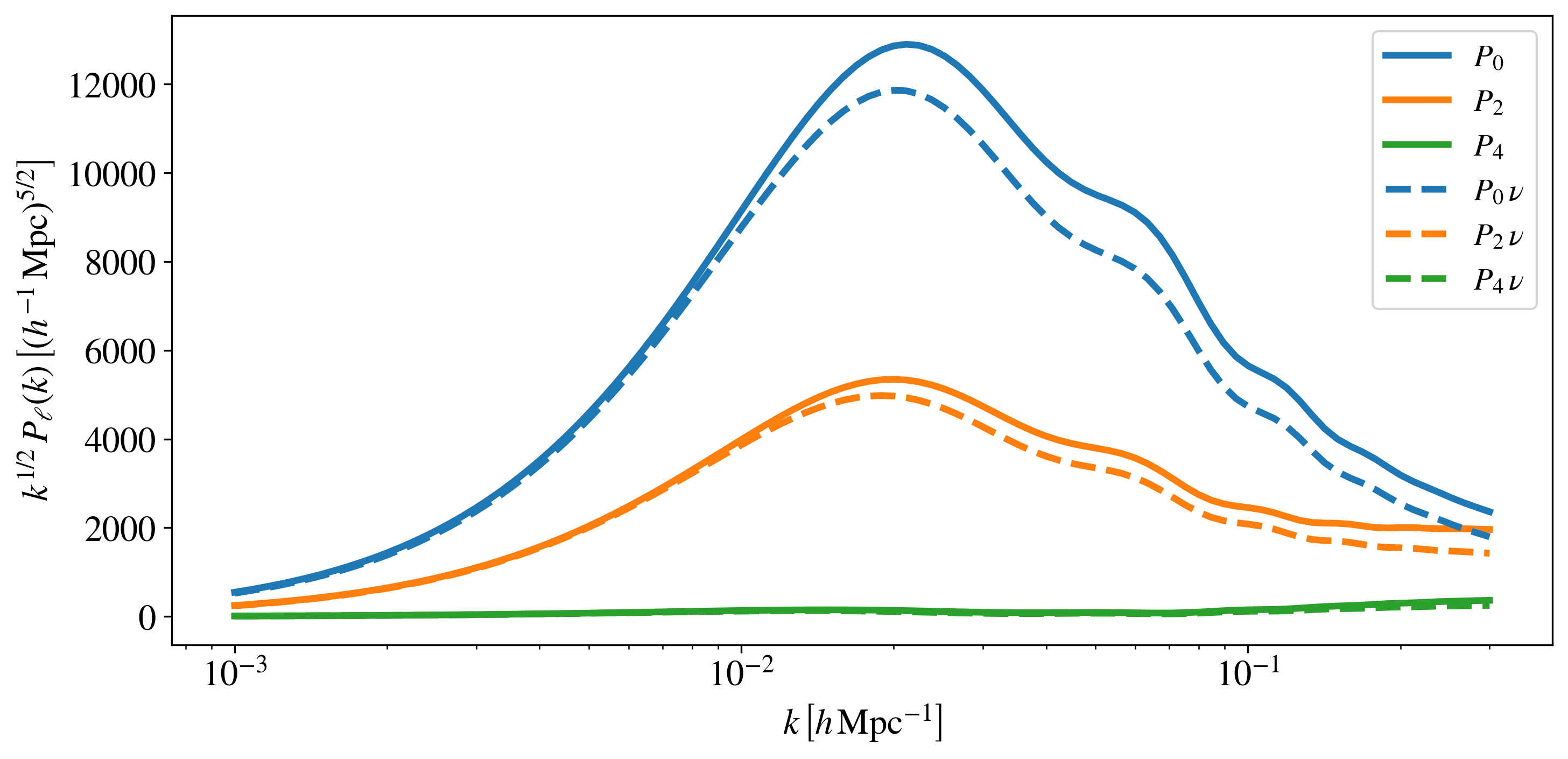
To check the differences, let’s plot the two sets of multipoles:

fig = plt.figure(figsize=(10,5))
ax = fig.add_subplot(111)
ax.semilogx(k_hMpc, k_hMpc**0.5 * Pell_LCDM['ell0'], c='C0', ls='-', lw=3, label=r'$P_0$')
ax.semilogx(k_hMpc, k_hMpc**0.5 * Pell_LCDM['ell2'], c='C1', ls='-', lw=3, label=r'$P_2$')
ax.semilogx(k_hMpc, k_hMpc**0.5 * Pell_LCDM['ell4'], c='C2', ls='-', lw=3, label=r'$P_4$')
ax.semilogx(k_hMpc, k_hMpc**0.5 * Pell_LCDM_nu['ell0'], c='C0', ls='--', lw=3, label=r'$P_0\,\nu$')
ax.semilogx(k_hMpc, k_hMpc**0.5 * Pell_LCDM_nu['ell2'], c='C1', ls='--', lw=3, label=r'$P_2\,\nu$')
ax.semilogx(k_hMpc, k_hMpc**0.5 * Pell_LCDM_nu['ell4'], c='C2', ls='--', lw=3, label=r'$P_4\,\nu$')
ax.set_xlabel(r'$k \, \left[h\,\mathrm{Mpc}^{-1}\right]$')
ax.set_ylabel(r'$k^{1/2} \, P_{\ell}(k) \, \left[(h^{-1}\,\mathrm{Mpc})^{5/2}\right]$')
ax.legend()
plt.tight_layout()
plt.show()

Advanced configuration options

In addition to the basic commands displayed in the previous section, COMET provides several alternative options/tools, like:

Specifying fiducial background cosmologies
Fixing Alcock-Paczynski parameters
Setting the shot-noise normalisation
Non-flat and non-\(\Lambda\) cosmologies
Using the \(f\)-\(\sigma_{12}\) parameter space
Using user-defined finger-of-god damping functions
Options for providing different \(k\)-scales, float vs np.array vs list and the corresponding outputs
Description of the fixed_cosmo_boost function, i.e., speedup when just changing bias parameters
Using different bases for galaxy bias
Using different counterterm definitions
Batch evaluation of multiple samples

Fiducial background cosmologies

In the previous section, we set the fiducial background cosmology by specifying the values of \(h\), \(\omega_b\), \(\omega_c\), and \(z\). Alternatively, we can directly provide the Hubble rate \(H_ {\rm fid}(z)\) and comoving transverse distance \(D_{m,\rm fid}(z)\) as follows:

H_fid = 135.0    # in units of km/s/(Mpc/h)
Dm_fid = 1490.0  # in units of Mpc/h

EFT.define_fiducial_cosmology(HDm_fid=[H_fid, Dm_fid])

Note that the units of \(H_ {\rm fid}(z)\) and \(D_{m,\rm fid}(z)\) are assumed to be in \(\mathrm{km\,s^{-1}\,Mpc^{-1}}\) and \(\mathrm{Mpc}\) (if use_Mpc=True), or \(\mathrm{km\,s^{-1}}\,(h^{-1}\,\mathrm{Mpc})^{-1}\) and \(h^{-1}\,\mathrm{Mpc}\) (if use_Mpc=False).

Note

We emphasize that the define_fiducial_cosmology function is used solely for setting the fiducial cosmological parameter values involved in computing the Alcock-Paczynski parameters. It does not set the default values for the evaluation of the model.

Alcock-Paczynski parameters

By default, the values of the Alcock-Paczynski parameters, \(q_{\parallel}\) and \(q_{\perp}\), are determined based on the provided cosmological parameters and fiducial background quantities (or the fiducial parameter dictionary). However, these values can be manually overwritten by specifying them explicitly as an argument in the Pell function:

q_para = 1.0
q_perp = 1.0

Pell_LCDM_noAP = EFT.Pell(k=k_hMpc, params=params, ell=[0,2,4], de_model='lambda', q_tr_lo=[q_perp,q_para])

This feature is particularly useful when one wishes to ignore Alcock-Paczynski distortions, as in the example above.

Shot-noise normalisation

By default, the shot noise parameters in the power spectrum model are expressed in units of \(L^3\) for NP0 and \(L^5\) for NP20 and NP22, where \(L = (\mathrm{Mpc})^3\) (use_Mpc=True) or \(L = (h^{-1}\mathrm{Mpc})^3\) (use_Mpc=False). It is possible to define a fixed normalisation scale (corresponding to the Poisson shot noise \(1/\bar{n}\)) by setting a sample number density as follows:

nbar = 1e-3  # in the respective units
EFT.define_nbar(nbar=nbar)

With this normalisation, NP0 becomes dimensionless, while NP20 and NP22 acquire units of \(L^2\). The same normalisation is also used for parameters entering the expression for the bispectrum (see below).

Non-flat and non-\(\Lambda\) cosmologies

Predictions for non-flat cosmologies can be obtained by simply specifying the curvature density parameter \(\Omega_k\) in the parameter dictionary:

params['Ok'] = 0.05

For alternative dark energy models, we need to specify the appropriate de_model argument in the Pell function.

For a non-evolving dark energy equation of state, we set de_model='w0'.
For a time-dependent equation of state in the standard CPL parametrisation (\(w_0\)-\(w_a\)), we set de_model='w0wa'.

In these cases, the corresponding values of \(w_0\) and \(w_a\) must be included in the parameter dictionary. For example:

params['w0'] = -1.1
params['wa'] = 0.1

We can now recompute the model using these updated parameter values and compare it with the standard flat :math:LambdaCDM prediction:

Pell_w0wa = EFT.Pell(k=k_hMpc, params=params, ell=[0,2,4], de_model='w0wa')

fig = plt.figure(figsize=(10,5))
ax = fig.add_subplot(111)
ax.semilogx(k_hMpc, k_hMpc**0.5 * Pell_LCDM['ell0'], c='C0', ls='-', lw=3, label='$P_0$, $\Lambda$CDM')
ax.semilogx(k_hMpc, k_hMpc**0.5 * Pell_LCDM['ell2'], c='C1', ls='-', lw=3, label='$P_2$, $\Lambda$CDM')
ax.semilogx(k_hMpc, k_hMpc**0.5 * Pell_LCDM['ell4'], c='C2', ls='-', lw=3, label='$P_4$, $\Lambda$CDM')
ax.semilogx(k_hMpc, k_hMpc**0.5 * Pell_w0wa['ell0'], c='C0', ls='--', lw=3, label='$P_0$, $w_0w_a$CDM')
ax.semilogx(k_hMpc, k_hMpc**0.5 * Pell_w0wa['ell2'], c='C1', ls='--', lw=3, label='$P_2$, $w_0w_a$CDM')
ax.semilogx(k_hMpc, k_hMpc**0.5 * Pell_w0wa['ell4'], c='C2', ls='--', lw=3, label='$P_4$, $w_0w_a$CDM')
ax.set_xlabel(r'$k \, \left[h\,\mathrm{Mpc}^{-1}\right]$')
ax.set_ylabel(r'$k^{1/2} \, P_{\ell}(k) \, \left[(h^{-1}\,\mathrm{Mpc})^{5/2}\right]$')
ax.legend(loc='upper left')
plt.tight_layout()
plt.show()

The \(f\)-\(\sigma_{12}\) parameter space

When calling the Pell function for a specific dark energy model (lambda , w0, w0wa), and based on the specific set of evolution parameters passed as input, the code automatically recalculates the values of s12, q_tr, q_lo, and f in the parameter dictionary. As a result, the internal values of these parameters (which can be accessed via EFT.params) are updated accordingly:

# s12, q_tr, q_lo and f are computed internally!
EFT.params
>> {'wc': 0.11544,
    'wb': 0.0222191,
    'ns': 0.9632,
    's12': 0.5644811904905519,
    'f': 0.7025465611424653,
    'b1': 2.0,
    'b2': -0.5,
    'g2': 0.0,
    'g21': 0.0,
    'c0': 0.0,
    'c2': 0.0,
    'c4': 0.0,
    'cnlo': 0.0,
    'NP0': 0.0,
    'NP20': 0.0,
    'NP22': 0.0,
    'NB0': 0.0,
    'MB0': 0.0,
    'h': 0.8,
    'As': 2.3,
    'Ok': 0.05,
    'w0': -1.1,
    'wa': 0.1,
    'z': 0.6,
    'q_tr': 1.081799699202137,
    'q_lo': 1.045999542223697}

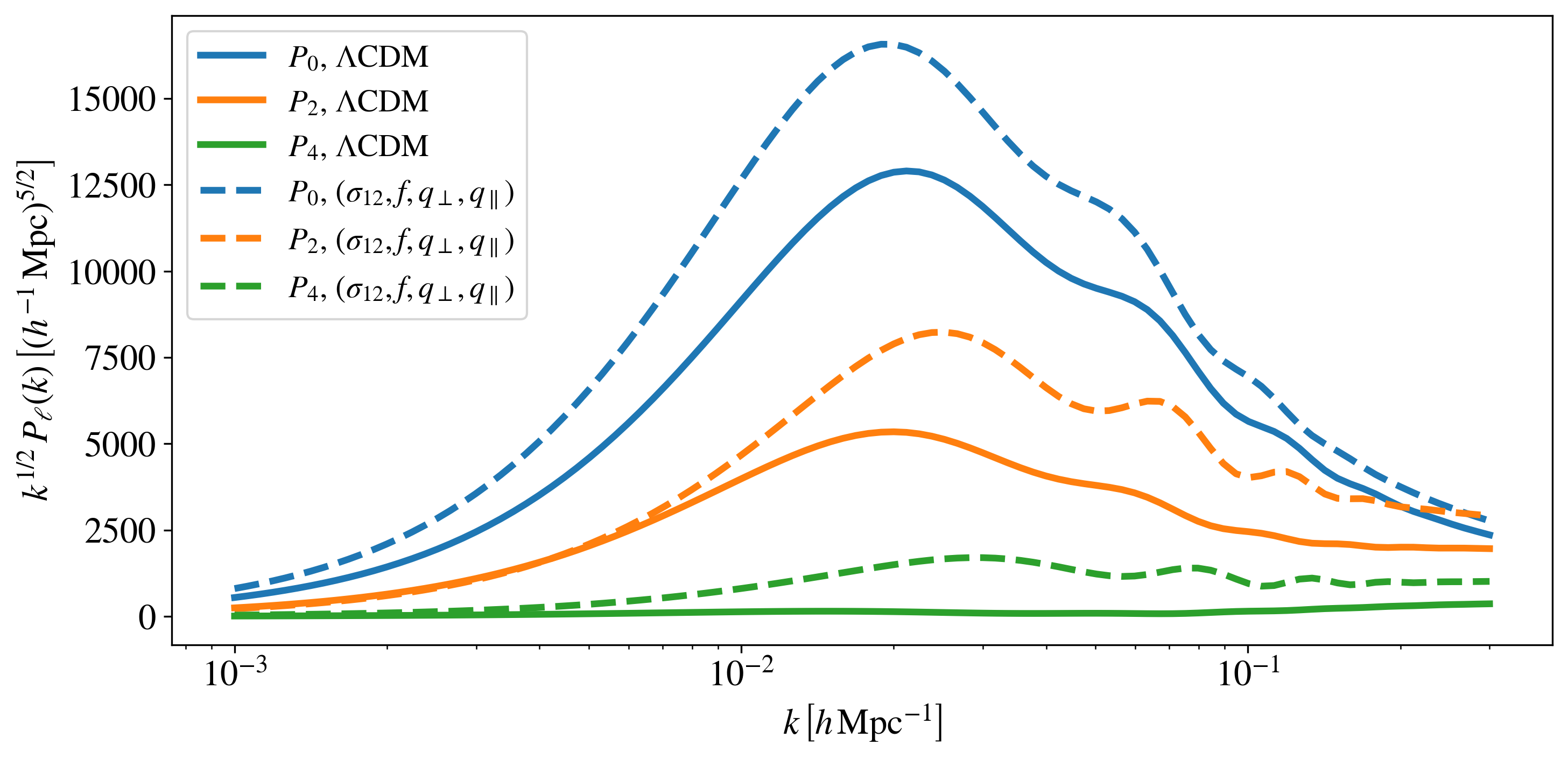
If we want to use the \(f\)-\(\sigma_{12}\) parameter space directly, we need to provide explicit values for s12, f, q_lo (\(q_{\parallel}\)) and q_tr (\(q_{\perp}\)). As an example, let’s redefine our parameter values:

# For predictions using the RSD parameter space we also need to specify values for the following four parameters, e.g.
params['s12']  = 0.6
params['q_lo'] = 1.1
params['q_tr'] = 0.9
params['f']    = 0.7

# When calling the Pell function, we do not specify a de_model
Pell_s12 = EFT.Pell(k_hMpc, params, ell=[0,2,4])

Note

When computing the multipoles using the \(\sigma_{12}\) parameter space and in \(h^{-1}\mathrm{Mpc}\) units, we need to specify a fiducial value for the Hubble rate (provided in the parameter dictionary). This is required to convert the native emulator output from \(\mathrm{Mpc}\) to \(h^{-1}\mathrm{Mpc}\) units.

Note

When computing the multipoles within the \(\sigma_{12}\) parameter space using the massive neutrinos emulators, the parameter dictionary must also contain a value of As, since this determines, jointly with s12, the amplitude of the neutrino suppression.

fig = plt.figure(figsize=(10,5))
ax = fig.add_subplot(111)
ax.semilogx(k_hMpc, k_hMpc**0.5 * Pell_LCDM['ell0'], c='C0', ls='-', lw=3, label=r'$P_0$, $\Lambda$CDM')
ax.semilogx(k_hMpc, k_hMpc**0.5 * Pell_LCDM['ell2'], c='C1', ls='-', lw=3, label=r'$P_2$, $\Lambda$CDM')
ax.semilogx(k_hMpc, k_hMpc**0.5 * Pell_LCDM['ell4'], c='C2', ls='-', lw=3, label=r'$P_4$, $\Lambda$CDM')
ax.semilogx(k_hMpc, k_hMpc**0.5 * Pell_s12['ell0'], c='C0', ls='--', lw=3, label=r'$P_0$, $(\sigma_{12}, f, q_\perp, q_\parallel)$')
ax.semilogx(k_hMpc, k_hMpc**0.5 * Pell_s12['ell2'], c='C1', ls='--', lw=3, label=r'$P_2$, $(\sigma_{12}, f, q_\perp, q_\parallel)$')
ax.semilogx(k_hMpc, k_hMpc**0.5 * Pell_s12['ell4'], c='C2', ls='--', lw=3, label=r'$P_4$, $(\sigma_{12}, f, q_\perp, q_\parallel)$')
ax.set_xlabel(r'$k \, \left[h\,\mathrm{Mpc}^{-1}\right]$')
ax.set_ylabel(r'$k^{1/2} \, P_{\ell}(k) \, \left[(h^{-1}\,\mathrm{Mpc})^{5/2}\right]$')
ax.legend(loc='upper left')
plt.tight_layout()
plt.show()

User-defined finger-of-god damping functions

By default, the VDG_infty model applies a damping function to both the power spectrum and bispectrum (see below). This function is derived from the resummation of quadratic non-linearities and depends on the parameter avir. However, users can override this default by supplying their own damping function via the W_damping argument in the Pellfunction. The corresponding function must accept two arguments, the scale \(k\) and the cosine \(\mu\) of the angle between the wave vector and the line of sight. For instance, to define a Lorentzian damping function, we can proceed as follows:

# Let's set up the VDG model first:
VDG = comet(model='VDG_infty', use_Mpc=False)
VDG.define_fiducial_cosmology(params_fid=params_fid)

# Define Lorentzian damping function
def W_Lorentzian(k, mu):
  sigma_v = VDG.params['avir'] # define velocity dispersion as a free parameter (reusing "avir")
  x = k * mu * VDG.params['f'] * sigma_v
  return 1.0 / (1.0 + x**2)

Hint

Note that model parameters can be accessed through the internal parameter dictionary of the VDG emulator object. It is (currently) not possible to define new model parameters, but existing parameters can be reused (if they are not used anywhere else in the model). When not using the default damping function, the parameter 'avir' is not required, so in the example above, we instead use it to allow for fits of the velocity dispersion.

We can now obtain predictions of the power spectrum multipoles with the Lorentzian damping function with the following call:

Pell_Lorentzian = VDG.Pell(k=k_hMpc, params=params, ell=[0,2,4], de_model='lambda',
                           W_damping=W_Lorentzian)

Providing different \(k\)-scales

There are multiple ways to specify the scales at which to compute the multipoles:

If passed as a scalar or a numpy array, all specified multipoles will be computed at those scales.
If passed as a list, the first entry of the list is evaluated for the first multipole, the second for the second multipole, and so on.

As an example, to compute the quadrupole at \(k = 0.1\,h\,\mathrm{Mpc}^{-1}\):

EFT.Pell(k=0.1, params=params, ell=2)
>> {'ell2': array([12734.58552054])}

To compute multiple multipoles at a given set of scales:

EFT.Pell(k=np.array([0.1,0.2,0.3]), params=params, ell=[0,2,4])
>> {'ell0': array([21993.36193293, 8421.42627781, 5055.15969128]),
    'ell2': array([12734.58552054, 7163.04358551, 5357.26768927]),
    'ell4': array([3027.98356766, 2244.35964221, 1870.99204263])}

To compute different multipoles at different scales:

EFT.Pell([np.array([0.1,0.2]),0.3], params, ell=[0,4])
>> {'ell0': array([21993.36193293, 8421.42627781]), 'ell4': array([1870.99204263])}

Note

If kmax is given as a list, its length must match the length of the specified multipoles (ell).

Hint

For better performance, it is recommended to compute all required multipoles and scales in a single function call rather than calling Pell multiple times for individual wavemodes.

Speed-up with fixed cosmological parameters

It is a common task to test the models at fixed cosmological parameters, and in that case COMET provides the function Pell_fixed_cosmo_boost, which accelerates the model computation. It computes all individual model contributions, which are kept fixed as long as the cosmological parameters are not changed, such that changing the bias parameters only is sped up drastically. In the following cells the differences on time can be seen, which reflects a speed up of around 3 orders of magnitude.

%timeit EFT.Pell(k_hMpc, params, ell=[0,2,4], de_model="lambda")
>> 5.19 ms ± 8.59 µs per loop (mean ± std. dev. of 7 runs, 100 loops each)

%timeit EFT.Pell_fixed_cosmo_boost(k_hMpc, params, ell=[0,2,4], de_model="lambda")
>> 9.46 µs ± 10.3 ns per loop (mean ± std. dev. of 7 runs, 100,000 loops each)

Note

Since the computation of all the individual contributions takes more time than the direct evaluation of the multipoles, this is really only useful at fixed cosmological parameters (or for samplers that can exploit a speed hierarchy).

Using different bases for galaxy bias

In COMET, the default galaxy bias expansion is the one proposed in Eggemeier et al. (2019), but it is also possible to specify other bias parametrisations:

Assassi et al. (2014), used e.g. in the analysis by Ivanov et al. (2019)
d’Amico et al. (2019)

The bias basis is defined at initialisation using the argument bias_basis, which accepts one of the followng strings:

'EggScoSmi' (for the Eggemeier et al. basis)
'AssBauGre' (for the Assassi et al. basis)
'AmiGleKok' (for the D’Amico et al. basis)

It is also possible to change the bias basis later via the function change_basis, e.g.:

EFT.change_basis(bias_basis='AssBauGre')

Changing the bias basis also changes the keys of the parameter dictionary that must be specified. The full list of available bias keys can be printed as follows:

print(EFT.bias_params_list)
>> ['b1', 'b2', 'bG2', 'bGam3', 'c0', 'c2', 'c4', 'cnlo', 'NP0', 'NP20', 'NP22', 'cnloB', 'NB0', 'MB0', 'cB1', 'cB2']

In this case we now need to provide values for 'bG2' and 'bGam3', i.e., parameters for 'g2' and 'g21' are now ignored. In case of the d’Amico et al. basis, we have:

EFT.change_basis(bias_basis='AmiGleKok')

print(EFT.bias_params_list)
>> ['b1t', 'b2t', 'b3t', 'b4t', 'c0', 'c2', 'c4', 'cnlo', 'NP0', 'NP20', 'NP22', 'cnloB', 'NB0', 'MB0', 'cB1', 'cB2']

Let’s change back to the default for the remainder of the tutorial:

EFT.change_basis(bias_basis='EggScoSmi')

Using different bases for counterterms

Apart from a different basis for galaxy bias, it is also possible to use a different definition of the counterterm parameters. This can either be done by providing the argument counterterm_basis at initialisation, or at any later point by calling the function change_basis. The currently supported specifiers are either:

'Comet': default choice, corresponds to definitions given in Eggemeier et al. 2023, 2025
'ClassPT': definitions adopted by the Class-PT code (Chudaykin et al. 2020)

Similarly to the previous case, the 'ClassPT' option changes the name of the keys of the internal parameter dictionary. The new names that must be passed as input are thus defined as:

EFT.change_basis(counterterm_basis='ClassPT')

print(EFT.bias_params_list)
>> ['b1', 'b2', 'g2', 'g21', 'c0*', 'c2*', 'c4*', 'cnlo*', 'NP0', 'NP20*', 'NP22*', 'cnloB', 'NB0', 'MB0', 'cB1', 'cB2']

Note

The parameter \(N_{P,0}\) is not modified since it has the same meaning in both parametrisations.

Again, let’s switch back to the COMET native basis:

EFT.change_basis(counterterm_basis='Comet')

Batch evaluation of multiple samples

In addition to the standard approach of computing a set of power spectrum multipoles for a given set of model parameters, COMET enables users to generate multiple sets in a single emulator call. This significantly reduces evaluation time compared to computing each set individually using the Pell function.

To enable this feature, simply provide NumPy arrays instead of scalar values for the various parameters, like:

params = {}

params['wc'] = np.array([0.11, 0.12, 0.13])
params['wb'] = np.array([0.021, 0.022, 0.023])
params['ns'] = np.array([0.92, 0.96, 1.00])

params['h']  = np.array([0.5, 0.7, 0.9])
params['As'] = np.array([1.5, 2.0, 2.5])
params['z'] = np.array([1.0, 1.5, 2.5])

params['b1'] = np.array([1.5, 2.0, 2.5])

Pell_LCDM = EFT.Pell(k_hMpc, params, ell=[0,2,4], q_tr_lo=[1.0,1.0], de_model='lambda')

The output of the Pell function remains a dictionary; however, in this case, the values are 2D arrays. The first dimension still corresponds to the wavemode \(k\), while the second dimension indexes the specific sample. It is implicitly assumed that the first values of all input parameters define the first sample, the second values define the second sample, and so on.

fig,axs = plt.subplots(1,3,figsize=(12,4))
for i in range(3):
  axs[i].semilogx(k_hMpc, k_hMpc**0.5 * Pell_LCDM['ell0'][:,i], c='C0', ls='-', lw=3, label=r'$P_0$')
  axs[i].semilogx(k_hMpc, k_hMpc**0.5 * Pell_LCDM['ell2'][:,i], c='C1', ls='-', lw=3, label=r'$P_2$')
  axs[i].semilogx(k_hMpc, k_hMpc**0.5 * Pell_LCDM['ell4'][:,i], c='C2', ls='-', lw=3, label=r'$P_4$')
  axs[i].set_xlabel(r'$k \, \left[h\,\mathrm{Mpc}^{-1}\right]$')
  axs[i].set_ylabel(r'$k^{1/2} \, P_{\ell}(k) \, \left[(h^{-1}\,\mathrm{Mpc})^{5/2}\right]$')
  axs[i].legend()
plt.tight_layout()
plt.show()

Note

The batch evaluation is not only limited to the power spectrum multipoles, but also to other output of COMET, such as the bispectrum multipoles, the linear power spectra, the \(\chi^2\) evaluation, etc. (see the rest of the tutorial).

Beyond \(P_{\ell}\) predictions

Below, we demonstrate several additional outputs that COMET can generate:

The linear power spectrum, both with and without infrared resummation.
The tree-level bispectrum multipoles.

Linear power spectrum

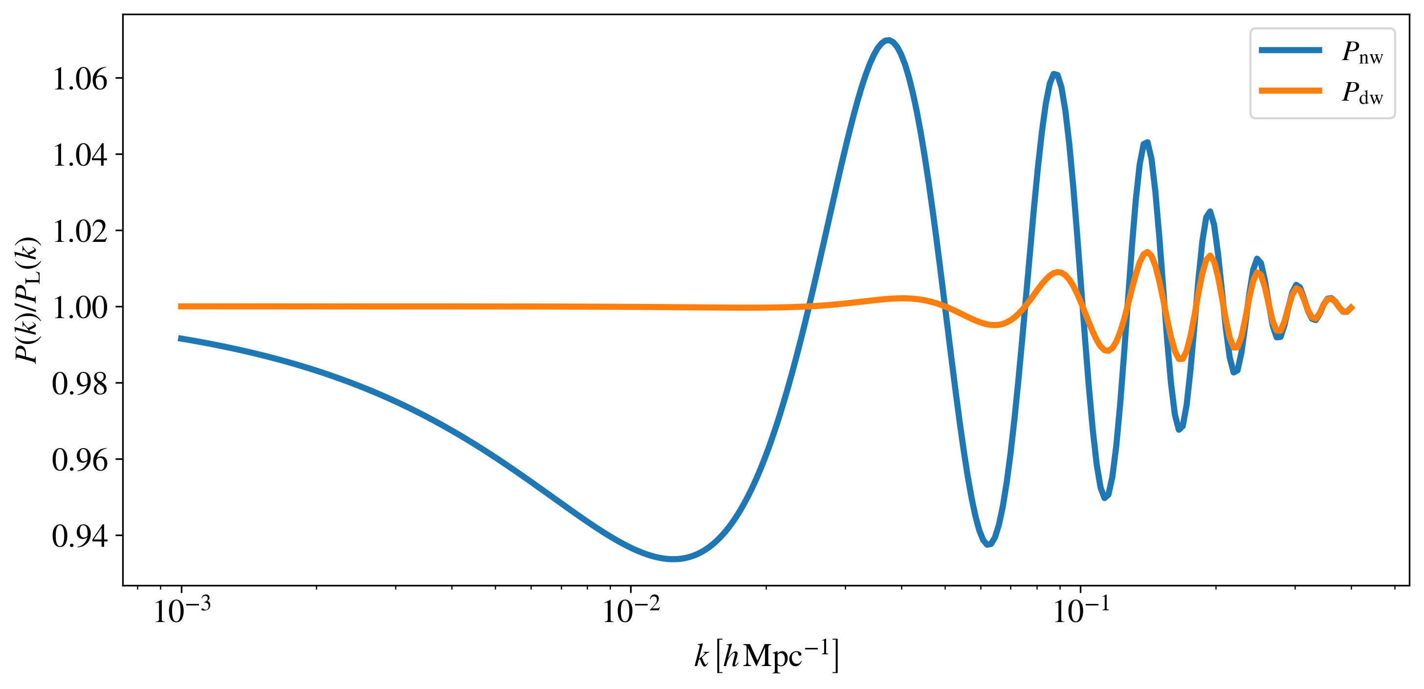
The linear power spectrum without infrared resummation (simply the emulated CAMB output) can be obtained using the function PL, while the linear power spectrum with damped BAO wiggles (infrared resummation) can be obtained using the function Pdw (note: this is not the smooth, no-wiggle power spectrum, which can instead be obtained using the function Pnw). The arguments for these functions are identical to those of Pell, except that a multipole number is no longer needed.

k = np.logspace(-3, np.log10(0.4), 300)
PL = EFT.PL(params=params, k=k, de_model='lambda')
Pnw = EFT.Pnw(params=params, k=k, de_model='lambda')
Pdw = EFT.Pdw(params=params, k=k, de_model='lambda')

Let’s plot the ratio of the no-wiggle and de-wiggled linear power spectrum over the linear power spectrum:

fig = plt.figure(figsize=(10,5))
ax = fig.add_subplot(111)
ax.semilogx(k, Pnw/PL, c='C0', ls='-', lw=3, label=r'$P_{\rm nw}$')
ax.semilogx(k, Pdw/PL, c='C1', ls='-', lw=3, label=r'$P_{\rm dw}$')
ax.set_xlabel(r'$k \, \left[h\,\mathrm{Mpc}^{-1}\right]$')
ax.set_ylabel(r'$P(k)\,/\,P_{\rm L}(k)$', fontsize=15)
ax.legend()
plt.tight_layout()
plt.show()

Tree-level bispectrum

COMET can also output the tree-level bispectrum (in real space, with the RS model) and its multipoles (in redshift space, with the EFT and VDG_infty models). These predictions are not emulated but are instead directly computed from the emulated de-wiggled power spectrum. To obtain the bispectrum, we use the function Bell. To demonstrate its usage, let’s first generate a set of triangle configurations:

k_hMpc_lin = np.arange(0.005, 0.3, 0.005)
tri = []
for i1,k1 in enumerate(k_hMpc_lin):
  for i2,k2 in enumerate(k_hMpc_lin[:i1+1]):
    for i3,k3 in enumerate(k_hMpc_lin[:i2+1]):
      if k2 + k3 >= k1:
        tri.append([k1, k2, k3])
tri = np.asarray(tri)

The Bell function has the same arguments and functionality as the analogous Pell function for the power spectrum. However, it requires the triangle configurations to be specified as a numpy array containing \(k_1\), \(k_2\), and \(k_3\) (currently, it is not possible to evaluate the multipoles for different triangles). Additionally, it includes the argument kfun, which is used to compress the number of unique math:k-modes. Ideally, this value should closely match the spacing between configurations (e.g., the bin width for measured data) but should not be much larger. If unsure, it’s best to choose a value significantly smaller than the typical spacing.

params['h'] = 0.69
params['z'] = 0.57
Bell = EFT.Bell(tri=tri, params=params, ell=[0,2,4], de_model='lambda', kfun=0.005)

Note

The initial call to Bell for a given set of configurations may take longer (depending on the total number of triangle configurations) since lookup tables are generated. However, all subsequent calls, even with different cosmological parameters, will be much faster. This means it is recommended to avoid calling Bell multiple times with different triangle configurations, and instead call it once for all the triangle configurations.

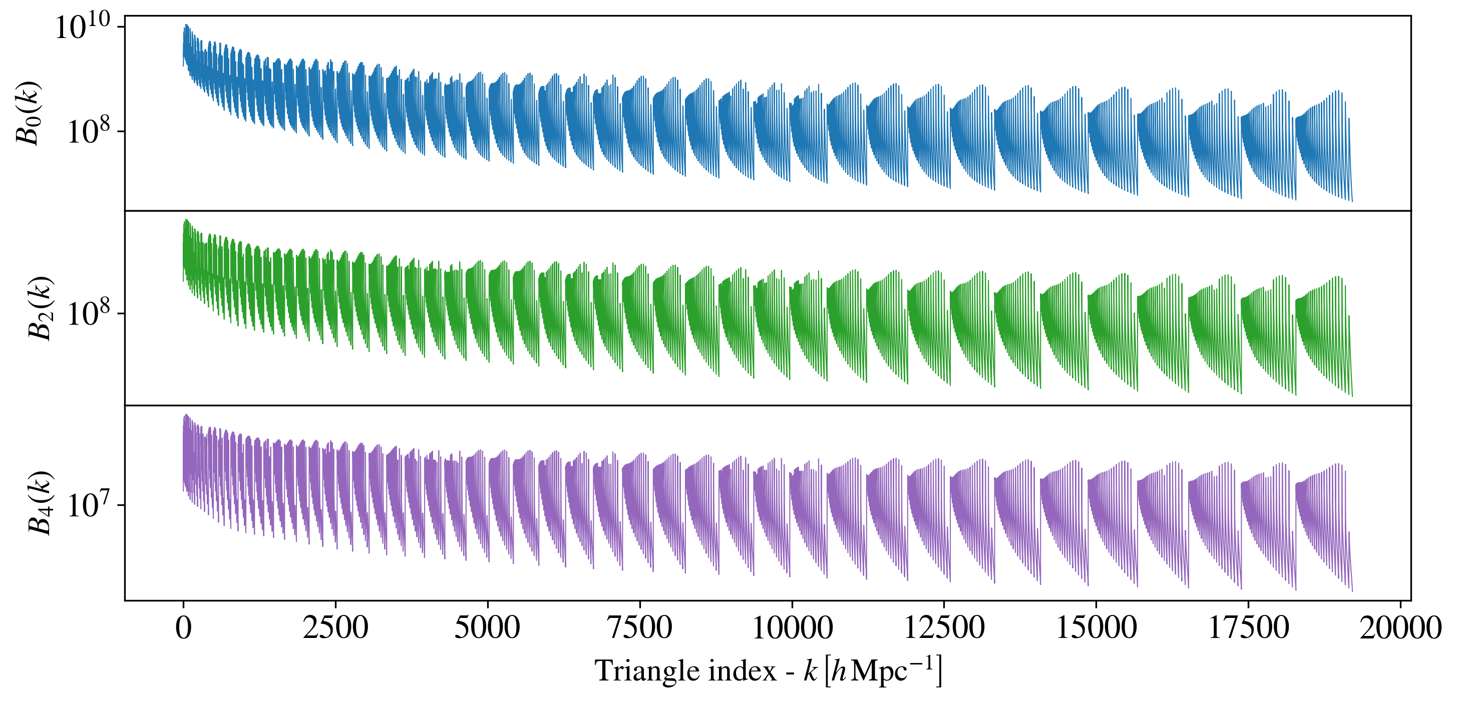
fig, axs = plt.subplots(3,1, figsize=(10,5), sharex=True)
for i in range(3):
  axs[i].semilogy(np.arange(tri.shape[0]), Bell['ell'+str(2*i)], c='C'+str(2*i), ls='-')
  axs[i].set_ylabel(f'$B_{i*2}(k)$',fontsize=15)
axs[-1].set_xlabel('Triangle index - $k \, \left[h\,\mathrm{Mpc}^{-1}\right]$', fontsize=15)
fig.tight_layout()
plt.subplots_adjust(wspace=0, hspace=0)
plt.show()

As in case of the power spectrum, it is possible to specify user-defined damping functions for the VDG_infty model. As arguments, it requires the list of triangle configurations, as well as (separately) the cosines of the angles between the three wave vectors and the line of sight. For example, for a Lorentzian damping function one can define:

def WB_Lorentzian(tri, mu1, mu2, mu3):
  kmu1, kmu2, kmu3 = VDG.get_kmu_products(tri, mu1, mu2, mu3)
  x2 = ((kmu1)**2 + (kmu2)**2 + (kmu3)**2) * (VDG.params['f'] * VDG.params['avirB'])**2
  return 1.0 / (1.0 + 0.5*x2)

Note

The products between the wave modes \(k_i\) and the cosines \(\mu_i\) are required in a specific format. For that purpose, one can use the provided get_kmu_products function.

In case of the EFT model, COMET provides two different counterterm prescriptions, which are either based on the definition in Ivanov et al. 2022 or Eggemeier et al. 2025. The default option is the latter, which defines a single counterterm parameter 'cnloB'. The former prescription can be enabled by calling the function

EFT.change_cnloB_type(type='IvaPhiNis')

in which case two counterterm parameters, 'cB1' and 'cB2', can be specified (see also here). To switch back to the default, one can call the same function with the specifier 'EggLeeSco':

EFT.change_cnloB_type(type='EggLeeSco')

Covariance matrices

In addition to computing power spectrum and bispectrum multipoles, COMET can also generate Gaussian covariance matrices for these statistics. The function structure is similar to that of Pell, having in common the arguments related to scales, parameters, multipole numbers, and the dark energy model. Additionally, the user must specify a bin width dk and a survey volume, both of which should be provided in the appropriate units. For example:

dk_hMpc = 0.005
k_hMpc_lin = np.arange(0.001, 0.3, dk_hMpc)
nk = len(k_hMpc_lin)
vol_hMpc = 3e9

Cov_hMpc = EFT.Pell_covariance(k=k_hMpc_lin, params=params, ell=[0,2,4], dk=dk_hMpc, volume=vol_hMpc)

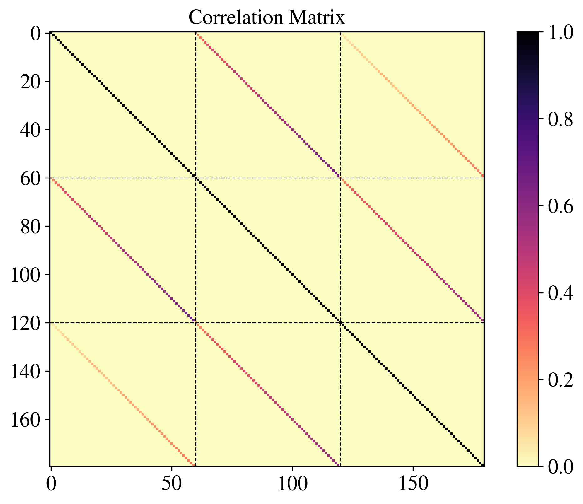
plt.figure(figsize=(9,6))
plt.title(r"")
plt.title(r"Correlation Matrix")
var_inv = np.diag(1.0 / np.sqrt(np.diag(Cov_hMpc)))
R_hMpc = var_inv @ Cov_hMpc @ var_inv
plt.imshow(R_hMpc, cmap='magma_r')
plt.axvline(nk, color='k', ls='--', lw='0.75')
plt.axvline(2*nk, color='k', ls='--', lw='0.75')
plt.axhline(nk, color='k', ls='--', lw='0.75')
plt.axhline(2*nk, color='k', ls='--', lw='0.75')
plt.colorbar()

The argument specifying the scales works similarly to how it does in the Pell function. It can be provided as either a single number or a numpy array, in which case all specified multipoles are evaluated at the same scales. Alternatively, it can be given as a list of numbers or numpy arrays, where each entry corresponds to the scales for the respective multipole in ell.

When explicitly specifying a dark energy model, the survey volume can be set in two ways. Instead of using the volume argument directly, one can alternatively define the minimum and maximum redshifts (zmin and zmax), the sky fraction (fsky), and a volume scaling factor (volfac) that defaults to 1. The total volume is then computed based on the chosen cosmological model. For example:

Cov_hMpc_LCDM = EFT.Pell_covariance(k=k_hMpc, params=params, ell=[0,2,4], dk=dk_hMpc,
                                    zmin=params['z']-0.1, zmax=params['z']+0.1, fsky=15000.0/(360**2/np.pi),
                                    volfac=1, de_model='lambda')

As a further extension, in the case when using measurements from a periodic box that have been averaged over different lines of sight, we have added the averaging corrections for the covariance matrix. We have created the flags avg_cov (set to False by default) and avg_los (set to 3 by default) for the Pell_covariance function, so that when avg_cov=True it by default will compute the average along the three perpendicular axes (x,y,z), but it is also possible to average over just 2 directions. Note that this computation is quite slow since it involves a different integral for each k-bin, it may be optimised in the future.

Similarly, we can compute the Gaussian covariance matrix of the bispectrum using the function Bell_covariance. Apart from the first argument, which specifies the triangle configurations (or a list of configurations for different multipoles), the arguments are identical to those of Pell_covariance. In addition, one can also specify kfun as in case of Bell (see above), which by default is set to the bin width dk. Let’s compute the bispectrum covariance matrix for a reduced set of triangle configurations with different scale cuts for the monopole, quadrupole, and hexadecapole:

id0p1 = np.where(tri[:,0] < 0.1)
id0p06 = np.where(tri[:,0] < 0.06)
id0p03 = np.where(tri[:,0] < 0.03)

# using the same scale cut for all multipoles
Cov_Bisp_hMpc = EFT.Bell_covariance(tri=tri[id0p1], params=params, ell=[0,2,4], dk=0.005, de_model='lambda',
                                    kfun=0.005, volume=3e9)

# using different scale cuts
Cov_Bisp_hMpc_diff_scale_cut = EFT.Bell_covariance(tri=[tri[id0p1],tri[id0p06],tri[id0p03]], params=params, ell=[0,2,4], dk=0.005, de_model='lambda',
                                    kfun=0.005, volume=3e9)

In the Gaussian approximation each block in the bispectrum covariance matrix is diagonal. Let’s plot these diagonals as a function of the triangle configuration index:

fig, axs = plt.subplots(2,3, figsize=(10,5), sharex=True, sharey=True)

ntri = id0p1[0].shape[0]

labels = ['$C_{00}$', '$C_{22}$', '$C_{44}$', '$C_{02}$', '$C_{04}$', '$C_{24}$']
colors = ['C0','C1','C2','C3','C4','C5']
for i in range(3):
    axs[0,i].semilogy(np.arange(ntri), np.diag(Cov_Bisp_hMpc[i*ntri:(i+1)*ntri,i*ntri:(i+1)*ntri]), c=colors[i], label=labels[i])
    axs[0,i].legend(fontsize=15)

n = 0
for i in range(2):
    for j in range(i,3):
        if i != j:
            axs[1,n].semilogy(np.arange(ntri), np.diag(Cov_Bisp_hMpc[i*ntri:(i+1)*ntri,j*ntri:(j+1)*ntri]), c=colors[n+3], label=labels[n+3])
            axs[1,n].legend(fontsize=15)
            axs[1,n].set_xlabel('Triangle Index',fontsize=15)
            n += 1

fig.tight_layout()
plt.subplots_adjust(wspace=0, hspace=0)

Hint

Note that both, Pell_covariance and Bell_covariance, allow also to specify the number of fundamental modes and fundamental triangles per bin, respectively. This is possible by using the optional arguments Nmodes and Ntri, which should be an array of the same length as either k or tri (and if either of these is given as a list, it should match the length of the longest entry in the list of scales or triangle configurations). If not provided, the following approximations are assumed when computing the covariance matrix:

\[\begin{split}N_{\rm modes} \approx \frac{V}{6 \pi^2}\,\left[\left(k+\frac{\Delta k}{2}\right)^3 - \left(k-\frac{\Delta k}{2}\right)^3\right]\,, \\[1.5em] N_{\rm tri} \approx \frac{V^2}{8 \pi^4}\,k_1\,k_2\,k_3\,\Delta k^3\,.\end{split}\]

Binning and discreteness effects

Power spectrum

Power spectrum multipoles are estimated in Fourier space from discrete grids of wave vectors, which means that a given multipole at scale \(k\) is an average over the discrete set of wave vectors \(\mathbf{q}\) whose magnitude falls into the spherical shell defined by \(k - \Delta k/2 \leq |\mathbf{q}| \leq k + \Delta k/2\). This leads to differences from the theory predictions, which (per default) assume continuous wave vectors and infinitesimally thin shells (\(\Delta k \to 0\)). However, the discreteness and finite bin width effects can be accounted for by averaging the anisotropic theory power spectrum over the same set of modes as those that are averaged over when performing the measurements.

In COMET, this can be done by specifying a binning dictionary, when calling Pell or Pell_fixed_cosmo_boost. In order to compute the set of discrete modes, it is necessary to know the size (i.e., the fundamental frequency) of the Fourier grid used for the measurements, as well as the bin width. These can be specified via the keys 'kfun' and 'dk' in the binning dictionary. For example:

binning = {'kfun':0.005, 'dk':0.005}

k = 0.005 + np.arange(80)*0.005
Pell_discrete = EFT.Pell(k=k, params=params, ell=[0,2,4], de_model='lambda', binning=binning)

Note

When calling Pell with the binning dictionary, the wavemodes specified via the argument k are assumed to be the bin centres.

Hint

Calling Pell for the first time with the binning dictionary takes a while longer as COMET has to find the set of discrete modes first. Subsequent calls (provided that the binning options or the maximum bin centre have not been changed) are much faster.

A common approximation to account for the finite bin width is to evaluate the power spectrum multipoles at the so-called effective wave modes, which are weighted averages over the discrete modes in a given bin. If one wants to evaluate the power spectrum multipoles at those effective modes, one can specify the additional key 'effective':True (False by default) in the binning dictionary; the wave modes specified via k are still supposed to correspond to the bin centres in this case.

Pell_discrete_eff = EFT.Pell(k=k, params=params, ell=[0,2,4], de_model='lambda',
                             binning={'kfun':0.005, 'dk':0.005, 'effective':True})

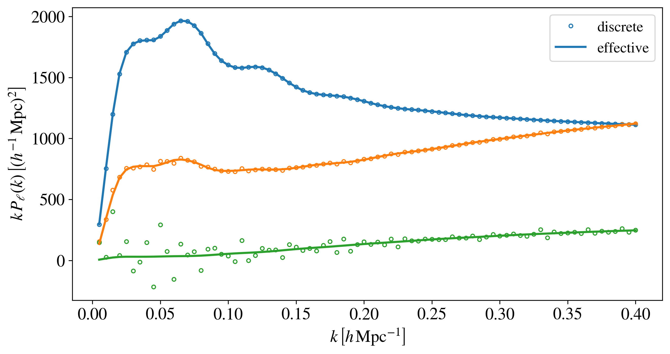
Let’s compare the two sets of predictions:

fig = plt.figure(figsize=(10,5))
ax = fig.add_subplot(111)

ax.plot(k, k * Pell_discrete['ell0'], m='o', c='C0', mfc='none', ms=3.5, label='discrete')
ax.plot(k, k * Pell_discrete['ell2'], m='o', c='C1', mfc='none', ms=3.5)
ax.plot(k, k * Pell_discrete['ell4'], m='o', c='C2', mfc='none', ms=3.5)

ax.plot(k, k * Pell_discrete_eff['ell0'], c='C0', label='effective')
ax.plot(k, k * Pell_discrete_eff['ell2'], c='C1')
ax.plot(k, k * Pell_discrete_eff['ell4'], c='C2')

ax.legend()
ax.set_xlabel(r'$k \, \left[h\,\mathrm{Mpc}^{-1}\right]$')
ax.set_ylabel(r'$k \, P_{\ell}(k) \, \left[(h^{-1}\,\mathrm{Mpc})^2\right]$')

plt.show()

Bispectrum

COMET also provides the possibility to correct for binning and discreteness effects in the bispectrum, using the approximation introduced in Eggemeier et al. 2025. Like for the power spectrum, the user can call the Bell function with a binning dictionary. However, there are a number of additional options available, which are summarised below:

binning = {
  'kfun': 0.005,                  # fundamental frequency of Fourier grid
  'dk': 0.015,                    # bin width
  'first_bin_centre': 0.0075,     # k-mode of first bin centre
  'do_rounding': False,           # apply rounding to fundamental configurations: True(default)/False
  'decimals': [3,3],              # defines rounding precision, default: [3,3]
  'shape_limits': [0.999,2.001],  # defines for which triangle configurations the binning/discreteness corrections are computed, default: [0.999,1.15]
  'fiducial_cosmology':{          # defines for which fiducial cosmology the corrections are computed, default: Planck2018 + redshift in parameter dictionary
    'h': 0.7, 'wc': 0.12,
    'wb': 0.022, 'ns': 0.96,
    'As': 2.2, 'w0': -1.0,
    'wa': 0.0, 'z': 0.5
  },
  'filename_root_kernels':'test'  # filename root to store binned tables
}

With the settings above, it is possible to define the triangle configurations for which the binning and discreteness corrections are being computed, as well as the efficiency (at the expense of accuracy). The 'shape_limits' property allows the user to specify a tuple of numbers [a,b], which select the following triangle configurations:

\[\frac{k_2+k_3}{k_1} < b \quad \land \quad \frac{k_2+k_3}{k_1} > a\]

In the following example with binning['shape_limits'] = [0.999,1.15] this corresponds to all triangle configurations between the two orange lines, i.e., triangle configurations that are closer to being equilateral (top right corner) are not considered for the binning correction.

fig = plt.figure(figsize=(5,3))
ax = fig.add_subplot(111)

x1 = np.linspace(0,0.5)
x2 = np.linspace(0.5,1)

ax.set_xticks(np.linspace(0,1,5))
ax.set_xlabel(r'$k_3/k_1$')
ax.set_xticklabels(['0.00','0.25','0.50','0.75','1.00'])
ax.set_yticks(np.linspace(0.5,1,3))
ax.set_ylabel(r'$k_2/k_1$')
ax.plot(x1, 1.-x1, c='k', lw=1)
ax.plot(x2, x2, c='k', lw=1)
ax.plot(np.concatenate((x1,x2)), np.ones(100), c='k', lw=1)
ax.set_xlim(-0.05,1.05)
ax.set_ylim(0.45,1.05)

shape_limits = [0.999, 1.15]
x3 = np.linspace(shape_limits[1]-1,shape_limits[1]/2)
x4 = np.linspace(shape_limits[0]-1,shape_limits[0]/2)
ax.plot(x3, shape_limits[1]-x3, c='C1', lw=3)
ax.plot(x4, shape_limits[0]-x4, c='C1', lw=3)

plt.show()

If one intends to compute the binning and discreteness corrections for all triangle configurations instead, one should set binning['shape_limits'] = [0.999,2.001].

The properties 'do_rounding' in combination with 'decimals' can be used to reduce the number of fundamental triangles over which the theory predictions have to be averaged in order to improve efficiency. For binning['decimals'] = [d1, d2] the discrete \(k_1,\,k_2,\,k_3\) and \(\mu_1,\,\mu_2,\,\mu_3\) values are approximated as follows:

\[\begin{split}k_i &\approx \left\lfloor 10^{d_1}\,\frac{k_i}{\Delta k} \right\rceil \, 10^{-d_1}\,\Delta k \\[0.5em] \mu_i &\approx \left\lfloor 10^{d_2}\,\mu_i \right\rceil \, 10^{-d_2}\end{split}\]

Note

The COMET binning module constructs the list of triangle configurations based on the first bin centre, the binwdith (both given in the binning dictionary), and the maximum k-mode given in the tri array when calling Bell. Currently, it assumes that the bin centres strictly form a closed triangle, i.e. \(k_1 \leq k_2 + k_3\) for \(k_1 \geq k_2 \geq k_3\).

Depending on the number of triangle configurations, the identification of the fundamental triangles and the averaging of the bispectrum kernel functions can be computationally demanding. However, for a given fundamental frequency, bin width and maximum k-mode, this only has to be performed once, such that the subsequent evaluation of the bispectrum model is very fast. For that reason, COMET allows to store any required information, such that at any later time (e.g., after re-initialising COMET), the computationally demanding steps can be skipped. By specifying the property filename_root_kernels one can set the root for the files that are generated, and when calling Bell again with the same binning dictionary, COMET will try to look for any existing files.

Note

This only works if all properties of the binning dictionary are identical. In particular, if files with a particular filename_root_kernels already exist, reusing the same name for a different set of binning options will lead to an error. In addition, the counterterm prescription that was used must also be identical.

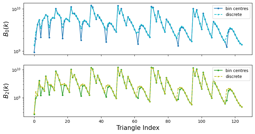
Let’s compare the bispectrum with and without the binning and discreteness corrections:

# define triangle configurations
k_hMpc_lin = np.arange(0.005, 0.05, 0.005)
tri =[]
for i1,k1 in enumerate(k_hMpc_lin):
    for i2,k2 in enumerate(k_hMpc_lin[:i1+1]):
        for i3,k3 in enumerate(k_hMpc_lin[:i2+1]):
            if i2 + i3 >= i1 - k_hMpc_lin[0]/binning['dk']:
                tri.append([k1, k2, k3])
tri=np.asarray(tri)

# let's evaluate with the parameters used in the fiducial cosmology
# (this means the binning/discreteness correction is exact)
for p in binning['fiducial_cosmology']:
    params[p] = binning['fiducial_cosmology'][p]

# evaluate bispectrum at the bin centres
Bell = EFT.Bell(tri=tri, params=params, ell=[0,2], de_model='lambda', kfun=0.005)

# evaluate bispectrum at the bin centres including the binning and discreteness corrections (this may take a few minutes)
Bell_discrete = EFT.Bell(tri=tri, params=params, ell=[0,2], de_model='lambda', kfun=0.005, binning=binning)

../_images/fig_bisp_centre_vs_discrete_02.png

As for the power spectrum, one can let COMET compute the effective triangle configurations for a given set of bin centres by adding binning['effective'] = True to the binning dictionary.

Warning

The bispectrum binning module requires the C++ library libgrid.so, which is compiled upon installation of COMET. If the automatic compilation failed, COMET will still load, but without the capability to use the bispectrum binning corrections. See here on instructions on how the library may be installed manually, if necessary.

When using the binning option in case of the "VDG_infty" model, the damping function is automatically expanded perturbatively, as otherwise the computation is too costly when varying cosmological parameters (or parameters of the damping function). One then has two options: 1) using the counterterm parameter 'cnloB' to describe the damping effect in the bispectrum, or 2) establishing a relation between 'cnloB' and any parameters appearing in the damping function. In the following we demonstrate the latter approach.

from scipy.optimize import curve_fit

# extend the range of triangle configurations to see an effect of the damping
k_hMpc_lin = np.arange(binning['first_bin_centre'], 0.14, binning['dk'])
tri =[]
for i1,k1 in enumerate(k_hMpc_lin):
    for i2,k2 in enumerate(k_hMpc_lin[:i1+1]):
        for i3,k3 in enumerate(k_hMpc_lin[:i2+1]):
            if i2 + i3 >= i1 - binning['first_bin_centre']/binning['dk']:
                tri.append([k1, k2, k3])
tri=np.asarray(tri)

# generate some realistic bispectrum covariance matrix
Bell_cov = EFT.Bell_covariance(tri=tri, params=params, ell=[0,2], dk=binning['dk'], de_model='lambda',
                               kfun=binning['kfun'], volume=3e9)

def compute_sv_avir_mapping(EFT, VDG, tri, params_fid, kf, cov_matrix,
                            navirB, nsv, sv_min=2, sv_max=10):
    """
       This function fits the bispectrum multipoles (monopole and quadrupole) from an
       expansion of the damping function to predictions that originate from the exact
       damping function for a range of 'avirB' and 'sv' values.

       Parameters
       ----------
       EFT: PTEmu object
          Comet instance of the EFT model (with default bispectrum counterterm prescription)
       VDG: PTEmu object
          Comet instance of the VDG_infty model
       tri: numpy.array
          Array of triangle configurations
       params_fid: dictionary
          Fiducial cosmological parameters (and linear bias) to use for the calibration
       kf: float
          Fundamental frequency
       cov_matrix: numpy.array
          Covariance matrix for the bispectrum multipoles
       navirB: integer
          Number of bins in 'avirB'
       nsv: integer
          Number of bins in 'sv'
       sv_min: float
          Minimum 'sv' value
       sv_max: float
          Maximum 'sv' value

       Returns
       -------
       avirB_list: numpy.array
          List of covered 'avirB' values
       sv_list: numpy.array
          List of covered 'sv' values
       mapping: numpy.array
          Corresponding coefficients for the mapping to 'cnloB'
    """
    def Bapprox(tri, a):
        params['cnloB'] = -a*VDG.params['avirB']**1.75 - 0.5*VDG.params['sv']**1.75
        B = EFT.Bell(tri, params, ell=[0,2], de_model='lambda', kfun=kf)
        return np.hstack([B[m] for m in B.keys()])

    params = {}
    for p in ['wc','wb','ns','h','As','z']:
        params[p] = params_fid[p]
    params['b1'] = params_fid['b1']

    avirB_list = np.logspace(-2,np.log10(10),navirB)
    sv_list = np.linspace(sv_min,sv_max,nsv)
    mapping = np.zeros((navirB,nsv))
    for i,avirB in enumerate(avirB_list):
        for j,sv in enumerate(sv_list):
            params['avirB'] = avirB
            VDG.params['sv'] = sv
            Bref = VDG.Bell(tri, params, [0,2], 'lambda', kfun=kf)
            Bref = np.hstack([Bref[m] for m in Bref])
            popt, pcov = curve_fit(Bapprox, tri, Bref, sigma=cov_matrix)
            mapping[i,j] = popt
    return avirB_list, sv_list, mapping

# this may take a few minutes; for realistic application one may want to
# increase navirB and nsv
avirB_list, sv_list, mapping = compute_sv_avir_mapping(EFT, VDG, tri, params, binning['kfun'], Bell_cov, 10, 10)

Let’s plot the coefficients as a function of 'sv' and 'avirB':

plt.imshow((np.log(np.abs(mapping))))
plt.ylabel('avirB',fontsize=15)
plt.xlabel('sv',fontsize=15)

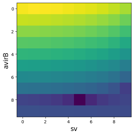
../_images/fig_cnloB_coefficients_02.png

Once we have this mapping, we can spline it and provide it to the Bell function:

from scipy.interpolate import RegularGridInterpolator
cnloB_spline = RegularGridInterpolator((avirB_list,sv_list), mapping)

# Going back to the smaller triangle configuration grid
k_hMpc_lin = np.arange(binning['first_bin_centre'], 0.05, binning['dk'])
tri =[]
for i1,k1 in enumerate(k_hMpc_lin):
    for i2,k2 in enumerate(k_hMpc_lin[:i1+1]):
        for i3,k3 in enumerate(k_hMpc_lin[:i2+1]):
            if i2 + i3 >= i1 - binning['first_bin_centre']/binning['dk']:
                tri.append([k1, k2, k3])
tri=np.asarray(tri)

for p in binning['fiducial_cosmology']:
    params[p] = binning['fiducial_cosmology'][p]
params['avirB'] = 4

VDG.params['wc'] = 0.1 # to trigger re-evaluation of the emulators in the call below (so that the 'sv' value is updated)
Bell_VDG = VDG.Bell(tri, params, [0,2], 'lambda', kfun=binning['kfun'])

binning['filename_root_kernels'] = 'test_VDG' # need to use a different filename root
Bell_VDG_discrete = VDG.Bell(tri, params, [0,2], 'lambda', kfun=binning['kfun'],
                             binning=binning, cnloB_mapping=cnloB_spline)

Note

The procedure above is just meant for demonstration - its accuracy still requires validation, which should be checked for any given realistic application.

Working with data sets

Loading data

We can load measurements of the power spectrum and bispectrum multipoles into COMET using the define_data_set function. This function takes first an identifier for the data set (obs_id; this can be anything, it will be used to reference the data) and any one of the following arguments:

stat. Can either be ‘powerspectrum’ or ‘bispectrum’; if not provided, stat is deduced from the number of columns in bins (see below).
bins. In case of the power spectrum: 1d-array of k-modes corresponding to the measurements; in case of the bispectrum: 2d-array with three columns corresponding to the triangle configuration (\(k_1\), \(k_2\), \(k_3\)) of the measurements.
signal. The measurements of the power spectrum or bispectrum; the size of the first dimension must match the size of bins, and it is assumed that the first column corresponds to the monopole, the second to the quadrupole, and the third to the hexadecapole (one does not need to provide all three multipoles, i.e., one can provide only the monopole, or monopole + quadrupole, but one cannot leave out preceding multipoles).
cov. The covariance matrix of the measurements, which must match the combined size of all given multipoles. If the dimension of cov is one-dimensional, it is assumed to be the diagonal of the covariance matrix.
theory_cov. A flag that specifies whether the given covariance matrix was derived analytically or from a set of simulation measurements. In the latter case an Anderson-Hartlap correction is applied to the inverse, based on n_realizations.
n_realizations. Number of realizations from which the covariance matrix was estimated, only used (and required) in case theory_cov=False.

Let us load some mock power spectrum measurements:

# Let's call this data set 'mock_Pk'
EFT.define_data_set(obs_id='mock_Pk', bins=k, signal=np.array([P0,P2,P4]).T, cov=Cov, theory_cov=False, n_realizations=300)

We can access the data through EFT.data['mock_Pk'] and check, for example, that the type of statistic was correctly identified (since it was provided above):

EFT.data['mock_Pk'].stat

Computing the \(\chi^2\)

Finally, we can let COMET directly compute \(\chi^2\) values based on the provided data set, a given set of model parameters and range of scales.

To do so, we call the function chi2, which takes as arguments the identifier of the data set, the parameter dictionary, a maximum k-mode value kmax, a model argument de_model. kmax can either be a number, in which case the same cutoff is applied for all multipoles, or a list of numbers for each individual multipole, as for the multipoles case. If the cutoff is zero (or smaller than the minimum scale of the observations) for a particular multipole, then it is excluded from the computation of the chi-square. kmax is also assumed to be in the units of the emulator. de_model can be one of the options specified before.

EFT.chi2(obs_id='mock_Pk',params=params, kmax=[0.30, 0.30, 0.30], de_model='lambda')
>> 6754.176546673202

Moreover, in order to speed up the computation of the \(\chi^2\), in the same way as Pell_fixed_cosmo_boost function, we can specify the flag chi2_decomposition in order to avoid recomputing the quantities depending on cosmological parameters. Let’s see how it works

%timeit EFT.chi2(obs_id='mock_Pk', params=params, kmax=[0.30, 0.30, 0.30], de_model='lambda', chi2_decomposition=False)
>> 6.37 ms ± 153 µs per loop (mean ± std. dev. of 7 runs, 100 loops each)

%timeit EFT.chi2(obs_id='mock_Pk',params=params, kmax=[0.30, 0.30, 0.30], de_model='lambda', chi2_decomposition=True)
>> 9.11 µs ± 20.6 ns per loop (mean ± std. dev. of 7 runs, 100,000 loops each)

It is also possible to compute the \(\chi^2\) for multiple data sets by giving chi2 a list of data identifiers. While in principle this could be useful to simultaneously analyse multiple power spectrum measurements at different redshifts, COMET currently does not support multiple parameter sets with different bias parameters, or at various redshifts (this will be possible in a future release). However, we can use this functionality to compute the joint \(\chi^2\) of the power spectrum and bispectrum.

As an example, let’s load some mock bispectrum data and store it in a new data container:

# data format: k1, k2, k3, B0, B0_var, B2, B2_var, B4, B4_var
data = np.loadtxt('mock_Bk_mean.dat')

EFT.define_data_set(obs_id='mock_Bk', bins=data[:,:3], signal=data[:,[3,5,7]], cov=np.hstack(data[:,[4,6,8]]), kfun=0.00166)

When providing a list of data identifiers, the kmax argument passed to chi2 can be a dictionary of \(k_{\rm max}\) values, where the keys must match the data identifiers. If not given as a dictionary, the same \(k_{\rm max}\) is used for each of the data sets. The following call of chi2 evaluates the \(\chi^2\) for the power spectrum and bispectrum data sets, using the power spectrum monopole and quadrupole up to \(k_{\rm max} = 0.3\) and \(0.25\,h\,\mathrm{Mpc}^{-1}\), respectively, and the bispectrum monopole and hexadecapole up to \(k_{\rm max} = 0.12\) and \(0.05\,h\mathrm{Mpc}^{-1}\):

EFT.chi2(obs_id=['mock_Pk','mock_Bk'], params=params, kmax={'mock_Pk':[0.3,0.25,0.], 'mock_Bk':[0.12,0.0,0.05]}, de_model='lambda')
>> 65495175908.83485

Note

The option chi2_decomposition is currently not available for the bispectrum.

Including analytical marginalisation

Some model parameters can be analytically marginalized when inferring cosmological parameters, in order to reduce the convergence time. This is possible for parameters that appear linearly in the theoretical model expression. In practice, this applies to \(\gamma_{21}\), \(c_0\), \(c_2\), \(c_4\), \(c_{\rm nlo}\), \(N_{P,0}\), \(N_{P,20}\), and \(N_{P,22}\).

To enable this functionality in COMET, simply specify the AM_priors argument when calling the chi2 function. This argument should be a dictionary where: - The keys correspond to the parameter names. - The values are lists of length 2, where the first element is the mean and the second is the standard deviation of the Gaussian prior used for the analytical marginalisation.

Let’s see an example:

EFT.chi2(obs_id='mock_Pk', params=params, kmax=[0.30, 0.30, 0.30], de_model='lambda', AM_priors={'g21': [0.0, 5.0], 'c0': [0.0, 100.0]})
>> 81718.03020579

Note

When working with a different bias or counterterm basis, it is intended that the marginalisation is done over the corresponding parameter set. In this case, the parameters specified in the AM_priors flags must be the ones of the selected basis.

Note

In case of a batch evaluation, the keys of the AM_priors dictionary must be the specific sample identifiers, similarly to what happens with the kmax flag. The value of each of these flags should be a dictionary like the one written above, with the possibility of analytically marginalising different parameters for different samples (or using different priors).

Convolution with survey window function

In order to compare the power spectrum model predictions to some actual measurements, we need to convolve with the survey window function. This can be done within COMET by providing a window function mixing matrix \(W_{\ell\ell'}(k,k')\) that connects the convolved and unconvolved power spectra via a simple matrix multiplication (see e.g. d’Amico et al. 2019):

\[P_{W,\ell}(k) = W_{\ell\ell'}(k,k') \cdot P_{\ell'}(k')\,,\]

where the summation over multipole numbers is implicit.

The mixing matrix and the associated scales for which it has been computed, \(k\) and \(k'\), can be specified via define_data_set using the arguments bins_mixing_matrix and W_mixing_matrix. The former is a list, containing the arrays for \(k\) and \(k'\). For example:

# Let's load some sample window function and k_prime values
W = np.fromfile('mock_Pk_window_W.npy').reshape((216, 4854))
k_prime = np.loadtxt('mock_Pk_window_kp.dat')

# The mixing matrix was computed for the following k-scales
k = np.arange(1,73)*2*np.pi/1500

# Load everything into COMET using the same data identifier as before ('mock_Pk')
EFT.define_data_set(obs_id='mock_Pk', bins_mixing_matrix=[k, k_prime], W_mixing_matrix=W)

We can now obtain the window-convolved power spectrum by passing the additional argument obs_id to Pell (the same functionality applies also to Pell_fixed_cosmo_boost) using the corresponding data identifier:

P_unconv = EFT.Pell(k, params, ell=[0,2,4], de_model='lambda')                  # unconvolved, equivalent with obs_id=None
P_conv = EFT.Pell(k, params, ell=[0,2,4], de_model='lambda', obs_id='mock_Pk')  # convolved with window function for data set 'mock_Pk'

f = plt.figure(figsize=(10,5))
ax = f.add_subplot(111)
ax.plot(k, k*P_unconv['ell0'],c='C0',ls='-',label='$P_{0}$')
ax.plot(k, k*P_conv['ell0'],c='C0',ls='--',label='$P_{W,0}$')
ax.plot(k, k*P_unconv['ell2'],c='C1',ls='-',label='$P_{2}$')
ax.plot(k, k*P_conv['ell2'],c='C1',ls='--',label='$P_{W,2}$')
ax.plot(k, k*P_unconv['ell4'],c='C2',ls='-',label='$P_{4}$')
ax.plot(k, k*P_conv['ell4'],c='C2',ls='--',label='$P_{W,4}$')
ax.set_xlabel('$k$ [h/Mpc]',fontsize=15)
ax.set_ylabel(r'$k\,P_{\ell}(k)$ [$(\mathrm{Mpc}/h)^{2}$]',fontsize=15)
ax.legend(fontsize=15,ncol=3)

We can also take the window function convolution into account when computing the \(\chi^2\). In that case we set the flag convolve_window=True (by default it is set to False):

EFT.chi2(obs_id='mock_Pk',params=params, kmax=[0.30, 0.30, 0.30], de_model='lambda', convolve_window=True)

This also works in combination with the option chi2_decomposition=True.